

Synthetic well logs generation via Recurrent Neural Networks
[ZHANG Dongxiao, CHEN Yuntian*  , MENG Jin]
, MENG Jin]
|
|


To supplement missing logging information without increasing economic cost, a machine learning method to generate synthetic well logs from the existing log data was presented, and the experimental verification and application effect analysis were carried out. Since the traditional Fully Connected Neural Network (FCNN) is incapable of preserving spatial dependency, the Long Short-Term Memory (LSTM) network, which is a kind of Recurrent Neural Network (RNN), was utilized to establish a method for log reconstruction. By this method, synthetic logs can be generated from series of input log data with consideration of variation trend and context information with depth. Besides, a cascaded LSTM was proposed by combining the standard LSTM with a cascade system. Testing through real well log data shows that: the results from the LSTM are of higher accuracy than the traditional FCNN; the cascaded LSTM is more suitable for the problem with multiple series data; the machine learning method proposed provides an accurate and cost effective way for synthetic well log generation.
Well logging is an essential tool for reservoir description and hydrocarbon resource evaluation. The integrated utilization of multiple geophysical logs in the borehole could greatly reduce the ambiguity of geologic interpretation and facilitate to construct convincible reservoir models for production. However, it is frequently the case that log information is missing or incomplete due to various inevitable causes, e.g., borehole enlargement, instrument failure, or incomplete logging out of economic concerns. The absence of these log records introduces major problems for reservoir studies. A common remedy is to re-log the well, but this is usually impractical and results in extremely high costs, especially when the well has been cased. Therefore, the reconstruction of missing and distorted wire-line logs is vital. For economic efficiency, a straightforward idea is to directly generate synthetic well logs with existing log data at hand, in which various approaches have been proposed. For example, one may synthesize the well logs according to geological and mechanic properties via certain physical models[1, 2]. However, the derived physical model always involves some degree of simplification, assumptions and subjective experiences, in which the quality of the synthetic well log curves cannot be guaranteed. An efficient alternative is to inspect the underlying and implicit correlations between different well logs. The missing logs are complemented according to their relationships with the extant logs. Certain approaches, such as cross-plot and multiple regression techniques, can be applied[3, 4]. Nevertheless, extremely complicated mapping exists between the non-linearly linked input and output well log data due to the heterogeneity and complex conditions underground. Thus, conventional approaches are incapable of constructing such sophisticated relationships since they are linearly derived and naive.
With the advent of machine learning applications in various fields of science and engineering in recent years, many researchers suggested using data-driven methods, e.g., supported vector machine (SVM), fuzzy logic models (FLM), and artificial neural networks (ANN), to deal with geological problems, e.g., geophysical parameter estimation[5, 6], lithology characterization[7, 8], stratigraphic boundaries determination[9, 10], etc. Specifically, the ANN is one of the research hotspots in recent years. Many researchers try to use ANN to generate well logs[11, 12, 13, 14, 15]. The networks in these applications are the traditional fully connected neural network (FCNN), which constructs a point-to-point mapping, which means that the output logs are only correlated to specific input logs at the same depth. However, the curvilinear trends and contextual information in reservoirs are neglected, which are critical in geological studies. Since the structure of FCNN is incapable of preserving previous information and fails to predict long-term series data, the quality of the generated well log is dubious. Even though researchers have integrated FCNN with other methods to solve this problem, e.g., wavelet transform[16] and singular spectrum analysis[17], the applications of these modifications are complicated and cumbersome. A better choice is to utilize the recurrent neural network (RNN)[18], in which an internal self-looped structure exists, allowing the network to remember previous information. The recurrent structure allows the data to flow both forward and backward within the network. Therefore, outputs of RNN are generated from a series of data inputs in consideration of their inner relationships and variation tendencies, which agrees well with the perspective of geological analysis.
In this study, the long short-term memory (LSTM) network[19], an advanced kind of RNN that is also a popular deep learning model, is introduced for synthetic well log generation. Since gate structures are constructed in self-looped neuron cells, the LSTM is able to preserve long-term previous information for future use without any further modifications. Such convenience and merit make the LSTM prevalent in artificial intelligence and deep learning, where the technique has been widely applied for nature language processing[20], machine translation[21], and speech recognition[22]. The RNN and the LSTM have also been applied in the field of hydrology to deal with time series data[23, 24]. However, to the best of our knowledge, no studies have yet applied such techniques for synthetic well log generation.
In this study, we aim to complement the missing or incomplete wire-line logs with synthetic well logs generated by the LSTM neural network. To better illustrate the details of the method, the theoretical foundations of the FCNN, RNN, and LSTM are introduced in the next section. The network architecture and specific settings are also discussed. We then test the method, in which real horizontal and vertical well log data are applied. We not only complement the well logs with missing parts based on partially available well logs in an auto-completion experiment, but also reconstruct the whole well logs based on nearby wells in a synthetic well log generation experiment. In addition, the LSTM results are compared with the traditional FCNN results of various depths. The outstanding performance of the LSTM demonstrates the accuracy and feasibility of the method for synthetic well log generation. Finally, conclusions and discussions are given.
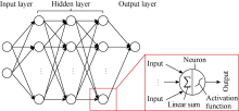
ANN is hierarchy model that is capable of approximating nonlinear functional relationships between input and output variables. From a mathematical perspective, a neural network can model any function up to any given precision with a sufficiently large number of basis functions[25, 26]. The FCNN is the most commonly used ANN, which has a typical hierarchical structure. The basic processing elements of FCNN are neurons, and they are organized in layers. In an FCNN, the neurons are fully connected to each other, which means that the neurons in a layer are connected to all of the other neurons in their adjacent layers. However, there is no connection among neurons in the same layer. A four-layer FCNN is illustrated in Fig. 1 as an example (the input layer is not counted in the number of layers). The output of a neuron is calculated by a nonlinear function of the sum of its inputs. The nonlinear function is also called the activation function, and the most popular choices are sigmoid, tansig, and ReLU[27]. The strength of the connections between different neurons are represented by weights, which adjust as learning proceeds. The FCNN has been widely utilized to solve many real-world engineering problems.
 | Fig. 1. Illustration of an FCNN with four layers. |
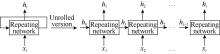
The FCNN performs well in many circumstances, but this network must accept a fixed-sized input and produce a fixed-sized output with a mapping using a determined amount of computational steps, which is very constrained. This characteristic limits the application of FCNN, especially to problems with sequential data[28]. In other words, FCNN cannot use its reasoning about previous events to inform later ones[29]. The recurrent neural network (RNN) has a loop in its architecture, which is used to transfer the influence of a former step to the current step. This architecture makes it possible for information to persist. Thus, RNN is capable to operate over sequences of vectors in inputs and outputs. A typical RNN is illustrated on the left side of Fig. 2. The xt and ht represent the input and output at step t, respectively. The arrows represent different matrix calculations. The loop is the main difference between RNN and the traditional FCNN. This loop enables information to be passed from one step to the next. This illustration of RNN is relatively ambiguous, and its unrolled version is easier to be understood, which is shown on the right side of Fig. 2. The RNN can be regarded as multiple copies of the same network, and the output of the former step is transferred to the next step. Thus, the output of RNN is influenced not only by the input of the current step, but also by the entire history of inputs fed into the model in the past. This chain-like nature of RNN reveals its advantage in sequence data analysis over other fixed networks. RNN is the natural network architecture to use with series data, such as well logs.
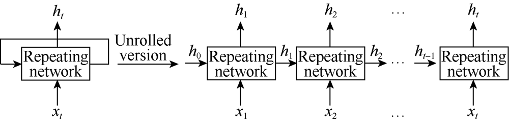 | Fig. 2. Illustration of standard RNN and its unrolled version. |
Regarding the calculation process of RNN, each layer computes the following function for each element in the input sequence:
${{h}_{t}}=\text{tanh}\left( {{w}_{\text{ih}}}{{x}_{t}}+{{b}_{\text{ih}}}+{{w}_{\text{hh}}}{{h}_{t-1}}+{{b}_{\text{hh}}} \right)$ (1)
As shown in Eq. 1, the hidden state at time t is determined not only by the input at time t, but also by the hidden state at time t-1. The final result at time t is generated based on the hidden state at time t. This usage of the hidden state increases the model’ s expressiveness, since the hidden state always has more dimensions and a wider value range than the original inputs. The hidden state helps the neural network express the complex distribution behind the limited observation value. The RNN possesses another feature, in addition to the loop in its architecture. The trainable parameters wih, whh, bih, and bhh in RNN are shared among different time steps. This idea of sharing parameters is the same as that of the convolutional neural network (CNN). Specifically, CNN shares convolution kernel parameters between spatial locations, while RNN shares parameters between the time steps of sequence data. Sharing parameters makes the model much less complex and allows the RNN to adapt to arbitrary-length sequences, resulting in better generalizability.
One of the advantages of the RNN is its ability to utilize information in previous steps to estimate the result in the present step. However, the RNN tends to exhibit poor performance in practice when the gap between the relevant information in the previous step and the present step becomes very large[30]. The LSTM is a particular type of RNN, which is designed to learn long-term dependencies. In fact, remembering information for long periods is the RNN’ s default behavior[29].
The LSTM has a similar form of a chain of a repeating network to the standard RNN. The repeating network in the standard RNN is very simple, while the LSTM has four interacting layers (three gate layers and a tanh layer), which is illustrated in Fig. 3. The cell state constitutes the key variable of the LSTM, which can pass through the LSTM, carrying information of previous steps. The gates are used to remove or add information to the cell state, according to the hidden state of the previous step and the input of the current step. The input of each repeating network includes the hidden state and the cell state from the previous step, and the input variable of the current step. The cell state is updated according to the results of the four layers. Finally, the updated cell state and hidden state constitute the output, which is sent to the next step.
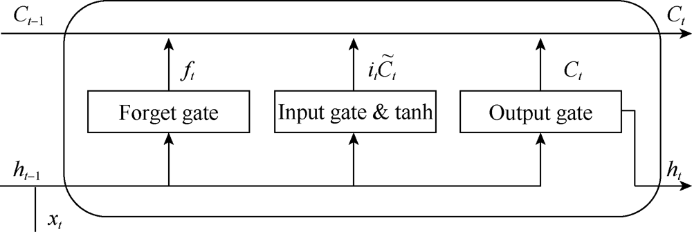 | Fig. 3. Illustration of the repeating network structure of the LSTM. |
The first layer is called the forget gate layer, which decides what information to forget. The forget gate is described by Eq. 2. The output ft is a number between zero and one, which will be multiplied with the cell state in Eq. 5. ft determines how much of the cell state from the previous step should be allowed to pass through.
${{f}_{t}}=\sigma \left[ {{W}_{\text{f}}}\left( {{h}_{t-1}}, {{x}_{t}} \right)+{{b}_{\text{f}}} \right]$ (2)
The second layer is called the input gate layer, which determines what new information should be stored in the cell state. The input gate is described by Eq. 3. The output decides which values in the third layer will be updated.
${{i}_{t}}=\sigma \left[ {{W}_{\text{i}}}\left( {{h}_{t-1}}, {{x}_{t}} \right)+{{b}_{\text{i}}} \right]$ (3)
The third layer is a tanh layer, which creates a new candidate value that could be added to the cell state. This layer is defined by Eq. 4:
${{\tilde{C}}_{t}}=\text{tanh}\left[ {{W}_{\text{c}}}\left( {{h}_{t-1}}, {{x}_{t}} \right)+{{b}_{\text{c}}} \right]$ (4)
After the preparation in the aforementioned three layers, the old memory carried by the old cell state Ct-1 is combined with the new candidate ${{\tilde{C}}_{t}}$, which is described by Eq. 5. The result from the forget gate ft decides what to forget in Ct-1, and the result from the input gate it decides what to add in ${{\tilde{C}}_{t}}$.
${{C}_{t}}={{f}_{t}}{{C}_{t-1}}\text{+}{{i}_{t}}{{\tilde{C}}_{t}}$ (5)
Finally, the last layer is called the output gate layer, which generates the output of the LSTM based on the updated cell state according to Eq. 6:
${{h}_{t}}=\sigma \left[ {{W}_{\text{o}}}\left( {{h}_{t-1}}, {{x}_{t}} \right)+{{b}_{\text{o}}} \right]\text{tanh}{{C}_{t}}$ (6)
The LSTM is a kind of RNN with four interacting layers in its repeating network. It is able to not only extract information from series data like the standard RNN, but also persist the information from previous time steps with long-term dependencies. The LSTM constitutes an ideal tool to generate synthetic well logs since the log data are series data and the trend of logs is significant. Moreover, long-term (spatial) dependencies exist in well logs since the sampling intervals are relatively small. The LSTM has sufficient long-term memory to solve these problems.
To test the performance of the LSTM, two computational experiments are carried out in this section, which are well log auto-completion experiment and synthetic well logs generation experiment. The main purposes of the experiments are: 1) to analyze the capability of the LSTM to auto-complete the well log curves with missing parts based on the incomplete logs themselves; 2) to evaluate the LSTM estimation accuracy of the synthetic well logs based on the information of nearby offset wells; and 3) to compare the performance of the LSTM with the traditional FCNN.
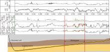
In this experiment, some parts of the well logs are missing. The LSTM method is utilized to regenerate and complete the well logs based on the remaining logs from the same well. A horizontal well from the Eagle Ford Shale in the U.S.A is taken as an example[31]. Five well logs are provided, which are gamma ray, array induction two-foot resistivity, neutron porosity, delta-time shear, and delta-time compressional. The logging section begins at 3719 m measured depth and ends at 5243 m measured depth, with a total length of 1524 m. As shown in Fig. 4, the logging section passes through two strata, and the boundary point of the stratum is at 4633 m. In this experiment, the neutron porosity, delta-time shear, and array induction two-foot resistivity in the depth range of 4 572 m to 4 877 m are removed to simulate the missing parts of log curves. The missing parts comprise 20% of the total logging section.
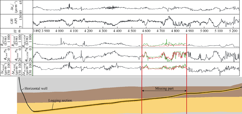 | Fig. 4. Auto-completed well logs and illustration of the horizontal well and the strata. |
The training dataset consists of two complete log sections, which are 3 719 m to 4 572 m and 4 877 m to 5 243 m. The log curve sampling intervals are 0.061 m (0.2 ft) and the length of the training sequence is set to 500, which equals 30.5 m (100 ft). This training length indicates an assumption that the data points within 30.5 m in front of each sampling point influence the value of the sampling point. By adjusting the training sequence length, the memory range of the LSTM can be modified according to real situations. The training sequences of the two complete log sections are separately extracted and then randomly mixed to construct the training dataset. Finally, there are a total of 19002 sequence data in the training dataset, each with a sequence length of 500, with gamma ray and delta-time compressional as inputs, and array induction two-foot resistivity, neutron porosity, and delta-time shear as outputs. The batch size is set to 100, i.e., 100 training data are randomly selected in each step of the training process. The LSTM model used in this experiment contains two LSTM layers and a fully connected layer. The hidden state of each LSTM layer has 30 dimensions. In order to avoid overfitting, dropout is applied to the LSTM with a drop probability of 0.3.
In the process of well log auto-completion, a small part of data before the missing segment is first selected as warm-up data, and the hidden state and the cell state of the LSTM are updated according to these data. Then, based on the updated hidden state and cell state, the predicted values of the missing logs are sequentially calculated. The specific process is illustrated in Fig. 5. The h0 and C0 in Fig. 5 are the initial hidden state and the cell state for the warm-up segment, respectively. The hd-1 and Cd-1 are the outputs of the warm-up segment, respectively, which are sent to the first step in the missing segment. Assuming that the first measured depth of the missing segment is d, the hidden state hd-1 and the cell state cd-1 can be calculated by the LSTM model based on the warm-up data at measured depth d-1. Then, based on the values of gamma ray and delta-time compressional at measured depth d, the hidden state hd and the cell state cd are predicted, and the array induction two-foot resistivity, neutron porosity, and delta-time shear at d are obtained. Finally, according to the hidden state and the cell state at d, combined with the input log curves at d+1, the hidden state and the cell state at d+1 are calculated, which generate the output log curves. In this well log auto-completion model, each prediction is based on the result of the previous step in the sequence, and the missing values are finally complemented one by one.
 | Fig. 5. Flow chart of the warm-up process. |
As shown in Fig. 4, the LSTM successfully extracts the patterns in the sequential data, predicts the missing segments, and completes the log curves based on these patterns. Regarding the delta-time shear and neutron porosity, the LSTM-based synthetic curves (green lines) and the real measured log curves (red lines) not only exhibit similar trends but also have similar values, indicating that the LSTM is capable to regenerate the missing parts of well logs. Concerning the array induction two-foot resistivity log, although the absolute value of the auto-completed curve is different from the actual log curve, a certain degree of similarity exists in the trend, which can be used as a reference of the missing segment. It can be seen that the auto-completed array induction two-foot resistivity curve and the real-world log curve differ greatly at the boundary of the strata. This may be due to the fact that the array induction two-foot resistivity is affected by oil content and salinity, and these effects are not well reflected in the input well logs. It is also possible that the array induction two-foot resistivity pattern at the strata junction is different from that in the upper and lower strata. It is challenging for LSTM to learn patterns at the boundary point of the stratum since it is not included in the training dataset. In general, when some parts of the well log curves are missing, the LSTM can be trained to identify patterns in the sequential log data based on the complete part in the same well. The missing segment can be regenerated according to these patterns learned by the LSTM, which means that the entire auto-completion process does not depend on other wells. However, performance may be significantly improved if complete logs are available in offset wells in the same field that can be used for learning.
In this section, synthetic well logs are generated using the LSTM, cascaded LSTM, and traditional FCNN, respectively, and the accuracy of these methods is compared. The data of this experiment come from six vertical wells (A1 to A6) in the Daqing Oilfield. Because vertical wells pass through more strata than horizontal wells, the mapping relationship between input and output logs is more complex, and this experiment is more challenging than the well log auto-completion experiment described in the previous section. In terms of training dataset, each vertical well contains seven logs, which constitute the amplitude difference of the micro potential and the micro gradient, the caliper, the spontaneous potential, the gamma ray, the high-resolution acoustic log, the borehole compensated sonic log, and the density. The first four log curves are used as input, and the last three curves are output. The logging section of A1 ranges from 780 m to 1 136 m in measured depth, A2 ranges from 795 m to 1 117 m, A3 ranges from 747 m to 1 059 m, A4 ranges from 920 m to 1236 m, A5 ranges from 842 m to 1 189 m, and A6 ranges from 716 m to 1007 m. In the process of constructing the training dataset, the training sequences of each well are independently extracted and then randomly mixed. The log curve sampling interval is 0.05 m, and the training sequence length is set to 500. Thus, when A1 to A6 are used to generate training data, the number of sequence data is 6 595, 5 919, 5 713, 5 791, 5797, and 5 295, respectively. The experiment employs the leave-one-out method, i.e., a total of six groups of experiments are performed. One of the six wells is used to construct a test dataset in each group of experiments, and the other five are combined into a training dataset. The well that is used as the test dataset is not subject to sequence extraction. Instead, the four input log curves are entered into the LSTM as four complete sequences to predict the other three output log curves. In terms of neural network architecture, the LSTM network uses two LSTM layers with a hidden state of 30 dimensions and two fully connected layers. Dropout is applied to the weights with a probability of 0.3. In addition, three FCNN with depths of 4, 8, and 12 layers are constructed as comparison models. The three FCNN have a similar number of weights to the LSTM network.
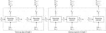
On the basis of the standard LSTM, this study also attempts to adopt an LSTM network with a cascade system. In this cascaded LSTM network, one of the unknown logs is first estimated from the known logs, and then the obtained synthetic log is combined with the known logs as new input, which is utilized to estimate another log from the remaining unknown logs. Finally, all of the unknown well logs are estimated by repeating the above steps. Taking the dataset in this experiment as an example, the high-resolution acoustic log curve is first estimated from the four known well logs. The obtained high-resolution acoustic log is then added to the input and used to predict the borehole compensated sonic log with the other four known well logs. Finally, the new input is constructed based on the high-resolution acoustic log, the borehole compensated sonic log, and the four known well logs to estimate the last unknown log (density). The entire process is illustrated in Fig. 6. This cascaded LSTM offers two advantages. First, because only one log curve is predicted at a time, mutual interference between output logs is reduced, which improves the accuracy of the model. Secondly, due to the adoption of the cascading idea, the model has greater input compatibility. For example, for a well with more known well logs, the model can be started directly from the middle step of the cascaded LSTM without retraining the model, which is beneficial to actual engineering deployments. The cascaded LSTM also possesses a drawback. Its network complexity is higher than that of the standard LSTM. However, since the dimensions of the input in synthetic well log generation problems are generally less than 10, even though the cascaded LSTM is more complicated, the amount of network parameters is still less than 50 000, which is much less than the commonly used deep neural networks with millions of weights. The complexity of the cascaded LSTM is acceptable considering currently available computational capability.
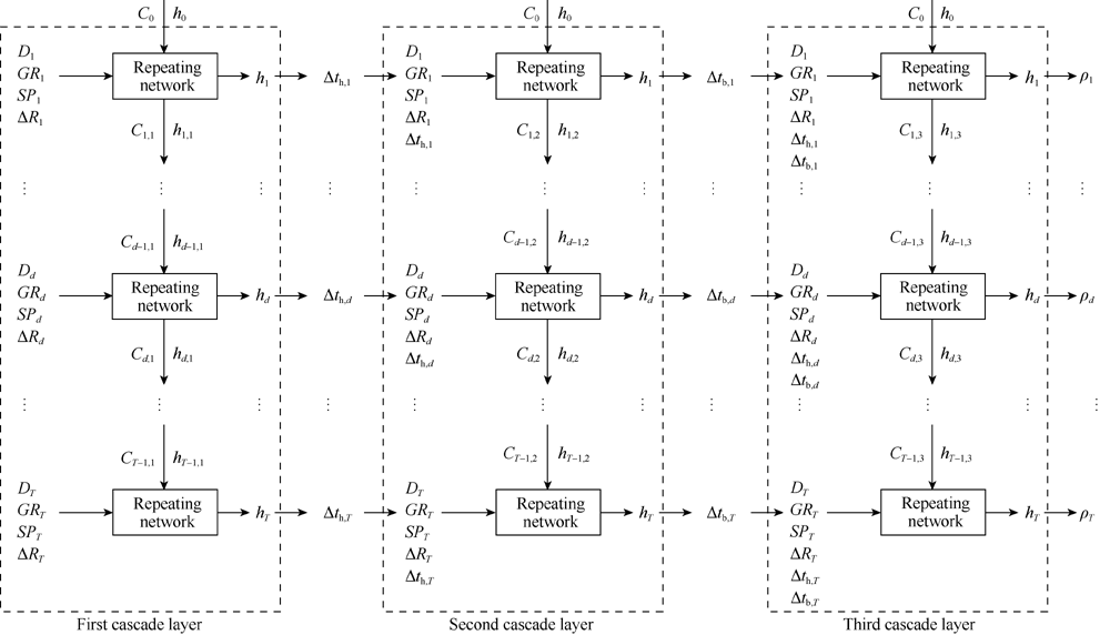 | Fig. 6. Architecture of the cascaded LSTM. |
In order to evaluate performance, the cascaded LSTM, standard LSTM, 4-layer FCNN, 8-layer FCNN, and 12-layer FCNN are applied to the synthetic well logs generation problem of the six wells in the Daqing Oilfield. The results are shown and compared in Table 1. The data in the table are the mean and standard deviation of the mean squared error (MSE) of the estimation values of different methods. Specifically, the smaller the MSE, the more accurate the model. Table 1 shows that the prediction results of the LSTM are more accurate than the 4-layer FCNN, 8-layer FCNN, and 12-layer FCNN. All of the five models achieve good estimations on the six wells, except for A2, which might result from that A2 has different hidden patterns from the other wells, and these patterns do not appear in the training dataset. However, the cascaded LSTM and standard LSTM still have acceptable accuracy on A2, which demonstrates their robustness to the unseen patterns. In addition, compared with the standard LSTM, the cascaded LSTM not only achieves higher prediction accuracy, but also has a significantly smaller standard deviation of prediction loss.
| Table 1 The mean squared error (MSE) of different models to regenerate the well logs from A1 to A6. |
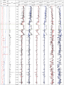
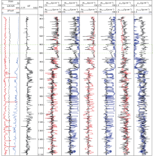
In order to analyze the performance of the cascaded LSTM, the synthetic logs of A3 and A2, which are the best and worst predictions of the cascaded LSTM, respectively, are plotted and compared with FCNN in Fig. 7 and Fig. 8. The left side of the depth ruler is the four known well logs, which are the amplitude difference of the micro potential and the micro gradient, the caliper, the spontaneous potential, and the gamma ray. The six log curves on the right side of the depth ruler correspond to the high-resolution acoustic log, borehole compensated sonic log, and density logs generated by the cascaded LSTM and the 8-layer FCNN, respectively. The red curves represent the results generated by the cascaded LSTM, the blue curves represent the results generated by the FCNN, and the black curves represent the real measured well logs as the reference. It is shown in the green dashed box in A3 (ranges from 820 m to 840 m) that the values of the high-resolution acoustic log and borehole compensated sonic log have a step increase in this interval. However, there are no obvious changes in the four input log curves within this interval, which makes the FCNN fail to generate this step change in its synthetic logs. Regarding the cascaded LSTM, since it is trained based on sequence data from offset wells, the cascaded LSTM can determine the high-resolution acoustic log and borehole compensated sonic log through the trend of the input curves in the depth range of 815 m to 820 m (red dashed box). According to the trend in the red dashed box before the green dashed box, the cascaded LSTM foresees the step increase at 820 m, which helps to generate the accurate synthetic logs in the range of 820 m to 840 m. This phenomenon reappears in the depth range of 860 m to 880 m of A2 in Fig. 8. This experiment indicates that the cascaded LSTM can comprehensively analyze the influence of data before the prediction point and the input at the prediction point. This characteristic enables the cascaded LSTM to accurately predict the trends of sequence data, such as synthetic well logs. Regarding A2, it is shown in Fig. 8 that both of the synthetic logs generated by the cascaded LSTM and FCNN have a large deviation from the real measured logs. Nevertheless, the cascaded LSTM still has better predictability for the overall trend of the target logs, as shown by the dashed green box. In addition, the FCNN is more unstable than the cascaded LSTM, which indicates that the cascaded LSTM is more robust when encountering data with unknown patterns.
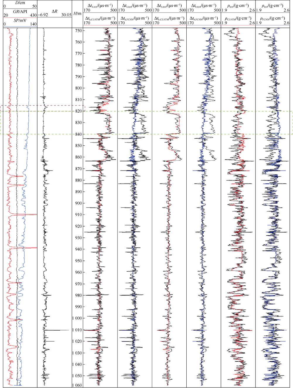 | Fig. 7. Synthetic well logs of A3 generated by the cascaded LSTM and FCNN (the best estimation result). |
 | Fig. 8. Synthetic well logs of A2 generated by the cascaded LSTM and the FCNN. |
The high accuracy and stability of the cascaded LSTM benefits from the fact that each stage of the prediction process uses the results as a new input in the next stage. This strategy not only assists to extract the patterns more effectively during the training process, but also use input information more efficiently in the forecasting process. When applying the cascaded LSTM, the prediction order of the unknown logs is significant. As the prediction result of each stage will become the input of the next stage, the prediction error will also be transferred to the next stage to a certain degree, leading to the problem of error accumulation. In response to this problem, it is recommended that simple log curves be predicted in shallow stages, and that complex log curves be progressively predicted as the stage deepens. In addition, the information contained in the results at shallow stages will be utilized by the deep stages to offset the influence of error accumulation. This method can achieve better results even in the deep-stage log curves, which is confirmed by the experimental data in Table 2. In the cascaded LSTM, the high-resolution acoustic log is first predicted at the first stage, the borehole compensated sonic log is then generated at the second stage with high-resolution acoustic log as one of the input logs, and finally the density log is generated. Although cumulative errors exist in the synthetic density log, the accuracy of the cascaded LSTM is higher than that of the standard LSTM, because the input of the cascaded LSTM has two more logs and contains more information than the standard LSTM.
| Table 2 Comparison of mean squared error (MSE) and standard deviation of the synthetic well logs generated by the cascaded LSTM and standard LSTM. |
In this study, the LSTM network in machine learning is used for log curve auto-completion and synthetic well logs generation. The LSTM can effectively extract patterns that have long-term spatial dependencies, and estimate and reconstruct the log curves based on these patterns. In addition, we also designed a cascaded LSTM by combining a cascade system with a standard LSTM. The cascaded LSTM outperforms the standard LSTM for problems with multiple series data (log curves).
In the well log auto-completion experiment, we utilized the LSTM to auto-complete the missing log curves of a horizontal well of the Eagle Ford Shale. 20% of the data in the log curves is lost, and the missing segment is at the junction of two strata through which the horizontal well passes. Because the log curves usually have different hidden patterns in different strata, the location of the missing segment increases the difficulty of this problem. However, the LSTM achieves satisfactory results. The training data in this experiment do not include the well logs of other offset wells, which means that the auto-completion process only relies on the log curves of the incomplete horizontal well itself.
In the synthetic well logs generation experiment, six vertical wells in the Daqing Oilfield are analyzed, and the standard LSTM is compared with three FCNN networks of different depths. A cascaded LSTM is also designed by combining the cascade system with the standard LSTM for solving problems with multiple related series data (well logs). In the cascaded LSTM, a relatively simple log curve is reconstructed at the shallow stage, and the result is used as a part of the input for the next stage. The predictions of the deep stages are based not only on the input logs in the training data, but also on the synthetic logs generated at the shallow stages. This method can extract information contained in the input more effectively, which improves prediction accuracy. This cascaded LSTM is particularly suitable for solving the problem of generating multiple well logs. The experimental results demonstrate that the cascaded LSTM offers a clear advantage in generating synthetic well logs, and the prediction results not only have smaller MSE, but also less uncertainty. This experiment is based on vertical wells. However, the cascaded LSTM is expected to do equally well or better for horizontal wells because the number of strata crossed by a horizontal well is less than that of a vertical well, leading to much simpler hidden patterns in the logs.
The method of auto-completing and generating well logs based on the LSTM proposed in this paper helps to reduce the cost of oil and gas development. In shale oil and shale gas development, well completion constitutes a significant portion of the total cost, whereas approximately 30% to 50% of the perforation clusters do not contribute to production[32]. In order to reduce the completion cost, it is necessary to increase our understanding of the formation through well logs. However, the current cost of well logging is high, and even more so for horizontal wells, for which the cost is approximately 10 times that in vertical wells[32]. The LSTM network proposed in this paper can solve this problem to a certain extent. The existing well logs in a block can be used to train the LSTM network. Then, for a newly drilled horizontal or vertical well, the complete set of logs can be automatically generated based on several available well logs and the LSTM network. The low cost of generating synthetic logs based on the LSTM makes it is possible to apply the LSTM on a large scale, which is conducive to assessment and analysis at the block and basin level. In addition, this LSTM-based synthetic well logs generation method can also be applied to log prediction while drilling. Real-time log curves are generated through real-time data collected during drilling, which can be utilized as reference information for adjusting the drilling process and designing completion strategies. Moreover, for blocks lacking well logs, existing models constructed for other blocks can be used based on transfer learning methods.
As a special kind of RNN, the LSTM is more suitable for generating synthetic well logs than the standard RNN and traditional FCNN. It is also possible to train the LSTM network based on a small number of wells, since it is capable to effectively extract information from a small training dataset. The LSTM is an accurate and cost-effective way for log auto-completion and synthetic log generation. This method enables us to obtain a better understanding of the formation and improve the design of drilling and completion strategies, which leads to lower costs and improved production in oil and gas development.
NomenclatureC— cell state;
Ct— cell state at step t;
${{\tilde{C}}_{t}}$— output of the tanh layer at step t;
d— index of the sampling point at the beginning of the missing segment;
D— caliper, cm;
ft— output of the forget gate layer at step t;
GR— gamma ray, API;
h— hidden state;
ht— hidden state at stept;
H— depth, m;
it— output of the output gate layer at step t;
L— length of the warm-up process;
Rat30— array induction two-foot resistivity, Ω · m;
Δ R— amplitude difference of the micro potential and the micro gradient;
SP— spontaneous potential, mV;
T— length of the missing part;
whh, bhh— hidden-hidden weights and bias, learnable;
wih, bih— input-hidden weights and bias, learnable;
Wc, bc— weights and bias of the tanh layer;
Wf, bf— weights and bias of the forget gate layer;
Wi, bi— weights and bias of the input gate layer;
Wo, bo— weights and bias of the output gate layer;
xt— input at step t;
Δ tb— borehole compensated sonic log, μ s/m;
Δ tco— delta-time compressional, μ s/m;
Δ th— high-resolution acoustic log, μ s/m;
Δ tsm— delta-time shear, μ s/m;
ρ — density, g/cm3;
σ — sigmoid function;
ϕ N— neutron porosity, %.
CLSTM— data generated via cascaded LSTM;
FCNN— data generated via FCNN;
LSTM— data generated via LSTM;
test— measured data (test data);
train— complete segment data that makes up the training data set.
The authors have declared that no competing interests exist.
| [1] |
|
| [2] |
|
| [3] |
|
| [4] |
|
| [5] |
|
| [6] |
|
| [7] |
|
| [8] |
|
| [9] |
|
| [10] |
|
| [11] |
|
| [12] |
|
| [13] |
|
| [14] |
|
| [15] |
|
| [16] |
|
| [17] |
|
| [18] |
|
| [19] |
|
| [20] |
|
| [21] |
|
| [22] |
|
| [23] |
|
| [24] |
|
| [25] |
|
| [26] |
|
| [27] |
|
| [28] |
|
| [29] |
|
| [30] |
|
| [31] |
|
| [32] |
|